Maths Methods 1&2 — Test Monday
This portal covers exactly what's on your test: Chapter 16 (Rates of Change — the prerequisite foundation), Chapter 17 (Differentiation of Polynomials), Chapter 18 (Applications of Differentiation), and Chapter 20A/20B (Chain Rule & Rational Powers). Content is pulled from your own Haileybury class notes and lecture videos, plus original worked examples and plain-English explanations to fill any gaps.
Study order suggestion
- Chapter 16 first — the prerequisite foundation. Average/instantaneous rate of change and basic kinematics, using only graphs and chords, before any differentiation rules exist. Everything after this chapter is really just a faster way to do what 16D already introduces by hand.
- Chapter 17 next — it's the toolbox (differentiation rules, limits, differentiability) everything else uses.
- Chapter 18 next — every lesson here is "take a derivative, then do something useful with it" (tangents, rates, stationary points, optimisation, kinematics).
- Chapter 20A/20B last — the chain rule and rational powers extend the same toolbox to composite functions and roots.
- Cram Sheet the night before, or the morning of.
Average Rate of Change
Plain English & method
CalculusThe branch of maths that studies rates of change — how fast one quantity changes as another one changes., in one sentence, is the study of rates of change — and this is the very first, simplest version of that idea, with no differentiation required yet.
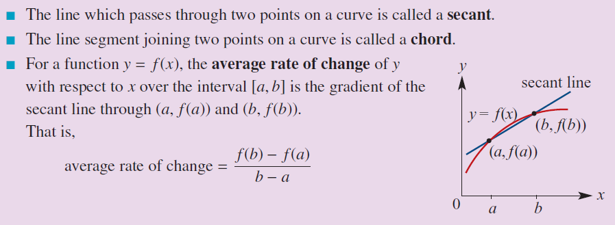
The average rate of change between two points P and Q on a curve is just the gradientHow steep a line is — its slope. Calculated as "rise over run": how far up divided by how far across. of the straight line joining P and Q (a chord) — the same "rise over run" slope formula from linear graphs, applied to two points that happen to sit on a curve instead of a straight line. Every time you see "gradient" from here on, read it as "steepness" or "slope" — they all mean exactly the same thing.
This tells you the overall trend between the two points — how much the function changed on average per unit of x — but says nothing about what happened in between (the function could have gone up, down, sped up, or slowed down along the way; the average rate of change only sees the two endpoints).
Key ideas (from class)
Class notes with a graph example (points P and Q on a curve) and a function-rule example, both computing the chord gradient.
Worked examples
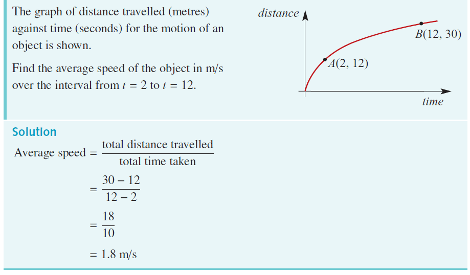
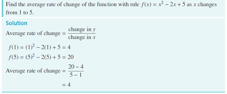
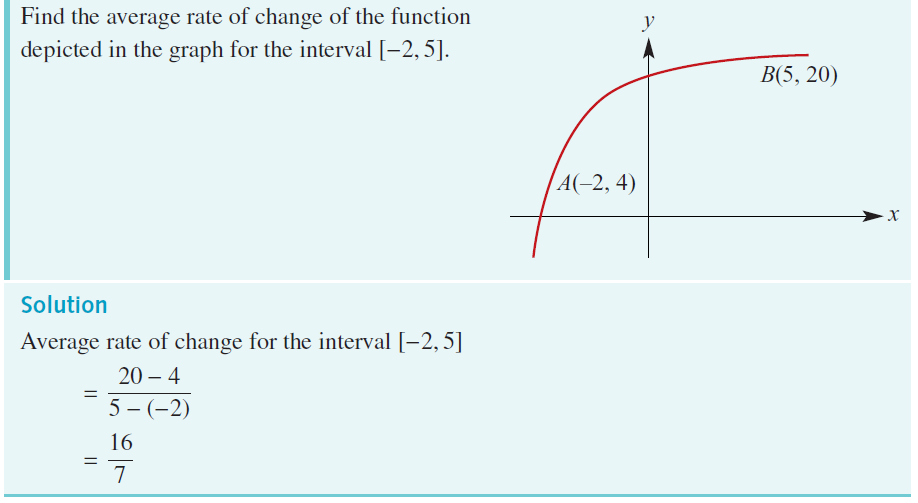
Worked examples from class: reading the average rate of change off a labelled graph, and calculating it directly from a function's rule between two given x-values.
Worked example (own): Find the average rate of change of \(f(x) = x^2 + 1\) between \(x = 2\) and \(x = 5\).
- \(f(2) = 4 + 1 = 5\), \(f(5) = 25 + 1 = 26\).
- \(\text{Average rate of change} = \dfrac{26 - 5}{5 - 2} = \dfrac{21}{3} = 7\).
- Average rate of change needs exactly two points — if a question gives you only one point, it's asking for something else (an instantaneous rate, 16D), not this.
- The units matter: if x is time in seconds and y is distance in metres, the average rate of change has units of metres per second — always attach the right units to the answer.
Instantaneous Rate of Change
Plain English & method
Unlike the average rate of change (16C), the instantaneous rate of changeThe rate of change at one single exact instant/point, rather than averaged over an interval. asks about the rate of change at one exact single point — this is the true starting idea behind everything in Chapter 17 (differentiation), just before any of the algebraic shortcuts get introduced.
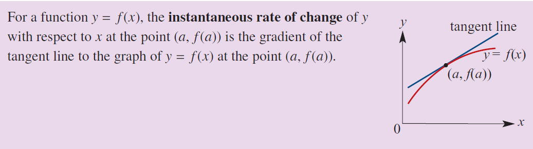
A tangentA straight line that touches a curve at one point and has the same gradient as the curve there. is a straight line that touches the curve at one point and has the same gradient as the curve at that exact point. Two ways to find the instantaneous rate of change at a point:
- Draw the tangent by hand at the point of interest, then calculate its gradient over a convenient interval (rise over run using two points on the tangent line itself). Quick, but only ever an estimate — how accurate it is depends entirely on how carefully the tangent is drawn.
- Use a short chord instead — pick a second point on the curve very close to the point of interest, and calculate the average rate of change (16C's method) between them. A chordA straight line segment connecting two points that both sit on the curve. between two very close points has almost the same gradient as the tangent at that point, so this gives a good numerical estimate without needing to draw anything.
This second method — shrinking the chord until it's almost the tangent — is exactly the seed idea that grows into the formal definition of the derivative in Chapter 17 (see 17B's "Building it from scratch" section for the full version of this idea, using dx instead of a fixed small gap).
Key ideas (from class)
Class notes and graph examples covering tangent-drawing and the chord-approximation method, including a worked question comparing average vs instantaneous rate at different points on the same graph.
Worked examples
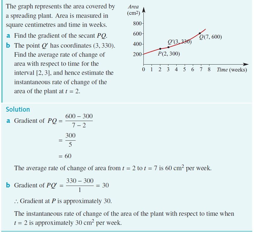
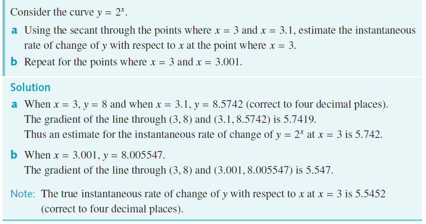
Worked examples: comparing the average rate of change over a wide interval against the instantaneous rate of change at specific points within it, and estimating a curve's gradient at a point using the gradient of a nearby short chord.
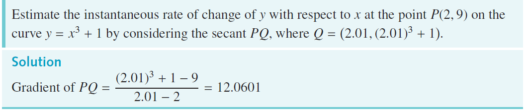
Worked example (own): Estimate the gradient of \(f(x) = x^2\) at \(x = 3\), using the chord from \(x = 3\) to \(x = 3.01\).
- \(f(3) = 9\), \(f(3.01) = 9.0601\).
- \(\text{Chord gradient} = \dfrac{9.0601 - 9}{3.01 - 3} = \dfrac{0.0601}{0.01} = 6.01\).
- This is very close to the true derivative value (\(2 \times 3 = 6\) from the power rule in 17B) — confirming that a short chord closely approximates the tangent's gradient.
- A tangent drawn by hand is only ever an estimate — if a question specifically says "estimate" or "approximately", it's expecting the hand-drawn-tangent or short-chord method, not an exact algebraic answer.
- The chord method gets more accurate the closer together the two points are — a chord between points far apart is a much rougher approximation of the tangent's true gradient.
Position and Average Velocity
Plain English & method
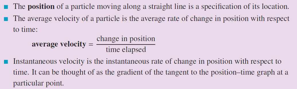
This lesson is the first appearance of kinematicsThe study of motion — here, always a single particle moving along a straight line. in the course — the same topic that returns properly, with full calculus, in 18F. Here, the ideas are introduced using only averages and graph-reading, before derivatives are available as a tool.
- Displacement describes an object's position relative to a fixed origin O. Positive displacement means the object is to the right of (or ahead of) the origin; negative displacement means it's to the left of (or behind) the origin.
- Velocity is the rate of change of displacement with respect to time — literally 16C/16D's "rate of change" idea, just with x(t) (position) as the function instead of a generic f(x).
- Acceleration is the rate of change of velocity with respect to time — the same idea again, one layer up.
Average velocity over a time interval is calculated exactly like 16C's average rate of change: (change in position) ÷ (change in time), i.e. \(\dfrac{x(t_2) - x(t_1)}{t_2 - t_1}\).
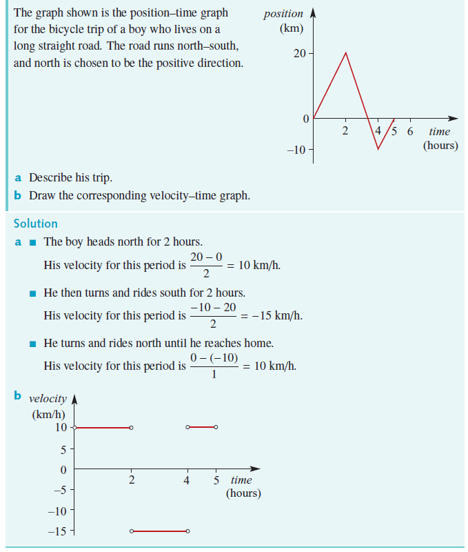
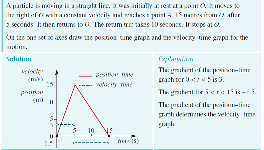
Reading motion graphs: on a position-time graph, the gradient at any point is the velocity at that instant. On a velocity-time graph, the gradient at any point is the acceleration at that instant. This is exactly why 18F later differentiates position to get velocity, and differentiates velocity to get acceleration — this lesson is building the graphical intuition for that before the algebra is introduced.
Key ideas (from class)
Class notes covering displacement/velocity/acceleration definitions, worked position-time graph description questions, and average-velocity calculation examples.
Worked examples
Worked examples: calculating average velocity over different time intervals from a position function, describing a bicycle trip from its position-time graph and sketching the matching velocity-time graph, and reading instantaneous velocity plus its sign (positive/negative) directly off a velocity function or graph.
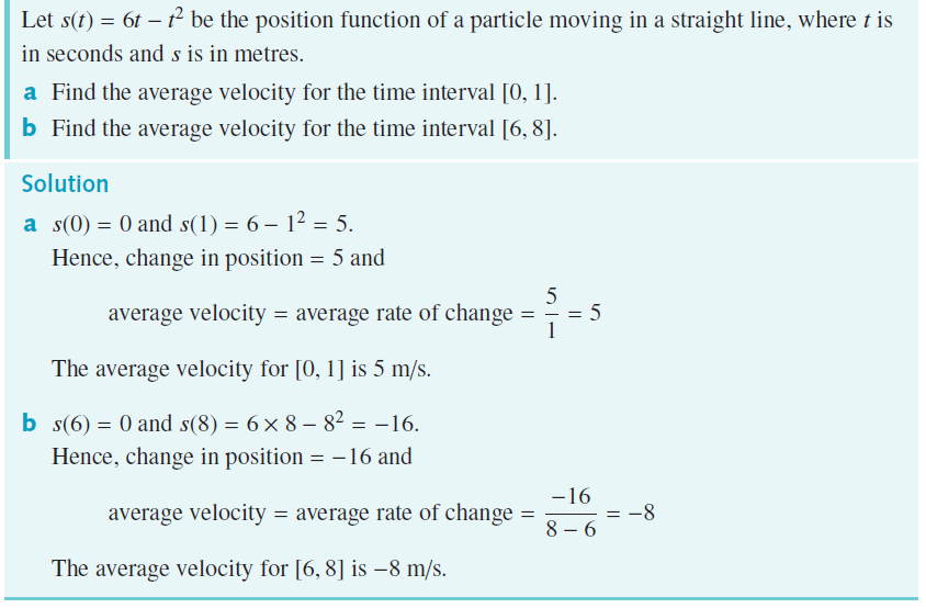
Worked example (own): A particle's position is \(x(t) = t^2 - 4t\) (metres, \(t\) in seconds). Find its average velocity between \(t = 1\) and \(t = 3\).
- \(x(1) = 1 - 4 = -3\), \(x(3) = 9 - 12 = -3\).
- \(\text{Average velocity} = \dfrac{x(3) - x(1)}{3-1} = \dfrac{-3-(-3)}{2} = \dfrac{0}{2} = 0 \text{ m/s}\).
- The average velocity is zero — the particle ended up back at the same position it started from over this interval, even though it moved in between.
- Positive velocity means moving in the positive direction (right/forward), NOT necessarily "speeding up" — speeding up vs slowing down is about acceleration, a separate question from direction.
- "Describe the trip" graph questions want the story in words (moving away, stationary, returning, at what approximate speeds) — read the gradient's sign and steepness at each section of the graph, don't just describe the graph's shape.
Rules for Differentiation
Plain English & method
Differentiation turns a function into a new function — its derivativeThe function giving the gradient (steepness) of the original curve at every point x. — that tells you the gradient of the original curve at every point. You almost never need first-principles limits to find it: there is a small toolbox of rules that let you differentiate a polynomial in seconds.
The power rule — the one rule that does 90% of the work: to differentiate \(ax^n\), bring the power down as a multiplier, then subtract 1 from the power.
Two shortcuts that follow immediately:
- The derivative of a sum is the sum of the derivatives — differentiate each term separately and add: d/dx[f(x) + g(x)] = f′(x) + g′(x).
- The derivative of a constant (a plain number with no x, like +7) is always 0 — a constant doesn't change, so it has zero gradient contribution.
Reading the formal notation
Every symbol in the formal definition of a derivative has one specific job — once you can name each part, the notation stops looking like a wall of unfamiliar signs:
| Symbol | What it means |
|---|---|
| f′(x) or dy/dx | "The derivative of f" — the gradient function itself, the thing you're solving for. |
| \(\lim_{h \to 0}\) | "The limit as h approaches 0" — what the expression settles down to as h shrinks toward (but never quite reaches) zero. |
| h | A tiny change in x — the gap between the two points used to build the chord (this is 16D's "short chord" idea, and Thompson's dx from the box above, just given a different letter). |
| f(x+h) | The function's value at the second point — x, nudged forward by h. |
| f(x+h) − f(x) | The change in the function's output — the "rise" between the two points. |
| [ f(x+h) − f(x) ] / h | The chord's gradient — "rise over run" between the two points, exactly 16C's average-rate-of-change formula. |

Your class notes write this using dx and dy instead of h (see the "Building it from scratch" box below); VCE exams and most textbooks use h. They're the same idea with different letters — if you see either form, recognise it as "take a tiny step, measure the resulting change, and see what the ratio settles down to as that step shrinks to nothing."
Building it from scratch (the Calculus Made Easy way)
The power rule feels like a magic trick if you only ever see the finished shortcut. It stops being magic once you build it yourself, the way Silvanus Thompson does in his 1910 book Calculus Made Easy: don't memorise the rule, watch it fall out of ordinary algebra.
Step 1 — nudge x forward by a tiny amount. Call that tiny nudge dx (read "dee-x"): not a variable multiplied by d, just the name for "a very small change in x". If \(y = x^2\), then nudging \(x\) to \(x + dx\) nudges \(y\) to some new value \(y + dy\). So:
Step 2 — expand the bracket, using ordinary algebra you already know, \((a+b)^2 = a^2 + 2ab + b^2\):
Step 3 — throw away the \((dx)^2\) term. This is the one genuinely new idea, and Thompson spends a whole chapter (his "orders of smallness") making it feel obvious rather than sneaky. If \(dx\) is already small — say a thousandth of \(x\) — then \((dx)^2\) is a thousandth of a thousandth: small squared, negligible compared to the plain dx term next to it. Picture a square of side x with a thin strip of width dx added to two sides: the strip areas are each roughly x·dx, but the tiny leftover corner square is \(dx \cdot dx\) — so small it's not even worth drawing. So we drop it:
Step 4 — subtract the original \(y = x^2\) from both sides, leaving just the changes:
Step 5 — divide both sides by dx to get the ratio of the changes — which is exactly what "the derivative" means, the gradient:
That's the whole derivation for \(x^2\) — no rule memorised, just expand, drop the tiny square, subtract, divide. Do the exact same four steps for \(y = x^3\) (expanding \((x+dx)^3\) instead) and you get \(dy/dx = 3x^2\); for \(y = x^4\) you get \(dy/dx = 4x^3\). Lay the results in a table and the pattern is obvious before anyone tells you the "rule":
| y | dy/dx |
|---|---|
| \(x^2\) | \(2x\) |
| \(x^3\) | \(3x^2\) |
| \(x^4\) | \(4x^3\) |
| \(x^n\) | \(n \cdot x^{n-1}\) |
The general power rule you use every day in this course is just that pattern, proven properly (it also works for negative and fractional powers, which is exactly what 17C and 20B rely on). Thompson even sanity-checks it with real numbers: at \(x=100\), \(x^2 = 10000\); nudge \(x\) up by \(dx=1\), and \((101)^2 = 10201\), so \(dy = 201\) for \(dx=1\) — close to \(2x = 200\), and the smaller you make dx, the closer that ratio gets to exactly 200. That numerical check is a genuinely useful way to convince yourself the rule is really true, not just asserted.
Key ideas (from class)
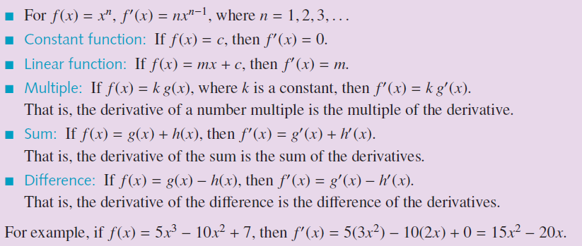
The key-ideas screenshot below is straight from your class notes — it states the power rule and the sum/constant rules exactly as you'll use them on the test.
Worked examples
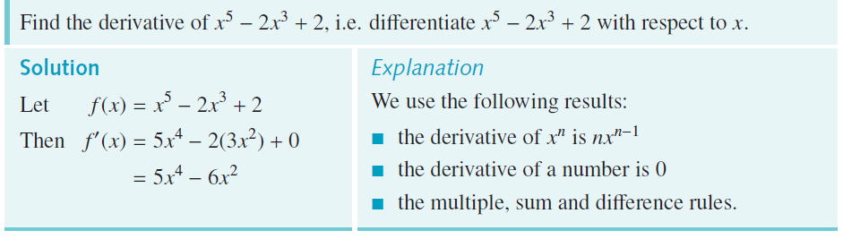
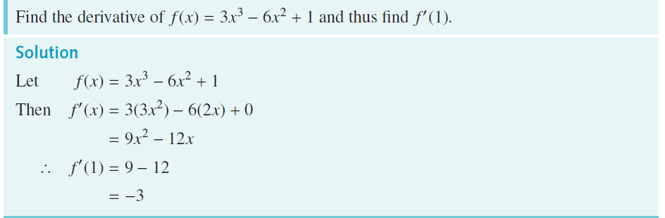
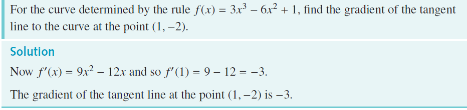
Two worked examples from your Haileybury notes: differentiating a simple polynomial term-by-term, and a case with a constant term dropping to zero.
Worked example (own): Differentiate \(f(x) = 3x^4 - 5x^2 + 7x - 9\).
- \(3x^4 \to 3 \times 4 \times x^3 = 12x^3\)
- \(-5x^2 \to -5 \times 2 \times x^1 = -10x\)
- \(7x \to 7 \times 1 \times x^0 = 7\)
- \(-9 \to 0\) (constant)
\(f'(x) = 12x^3 - 10x + 7\)
- Forgetting to drop the constant term to 0 — a lot of marks are lost writing "+7" instead of "+0" at the end of a derivative.
- The power rule needs the term in the form \(ax^n\) first — expand brackets before differentiating if the function isn't already in that form.
Differentiating xⁿ (negative powers)
Plain English & method
The power rule from 17B still works exactly the same way when the power is negative — bring the power down, subtract 1. The only new thing is domainThe set of x-values a function is actually allowed to take.: a negative power means x is in a denominator (e.g. \(x^{-2} = 1/x^2\)), and you can never divide by zero, so x = 0 has to be excluded from the domain of both the function and its derivative.
Rewriting the domain rule concretely from your notes:
- If n is positive, the domain of \(x^n\) is all real numbers (no restriction).
- If n is negative, the domain of \(x^n\) is \(x \neq 0\) (x can be anything except zero).
Key ideas (from class)
Class notes cover differentiating negative-power terms and stating the correct domain alongside the answer.

Worked examples
Worked examples: finding a derivative with a negative power, evaluating a derivative at a given x-value, and finding a gradient at a specific point on the curve.
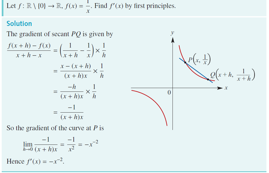
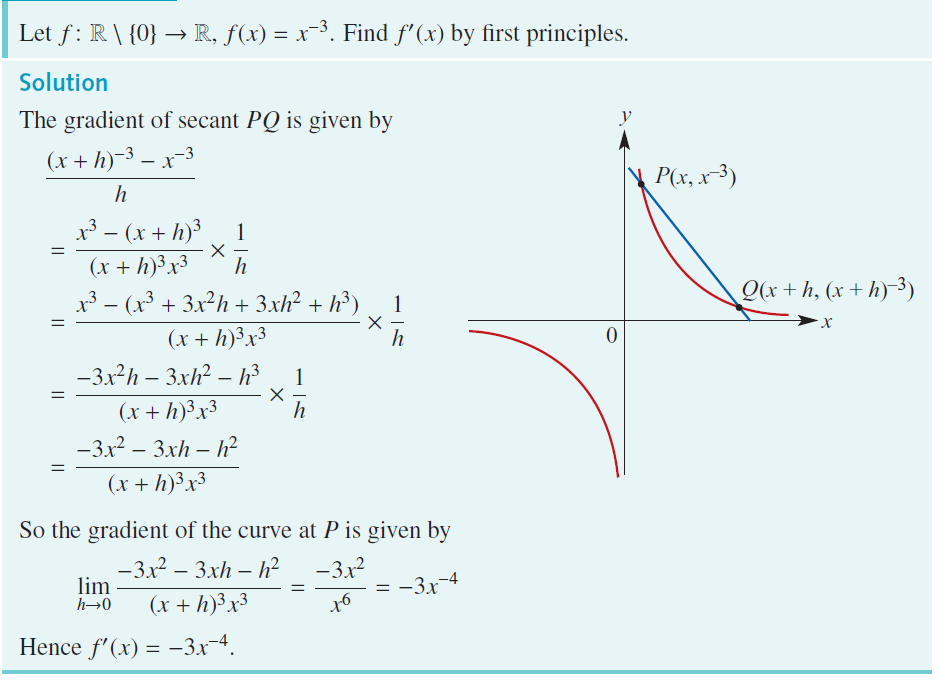
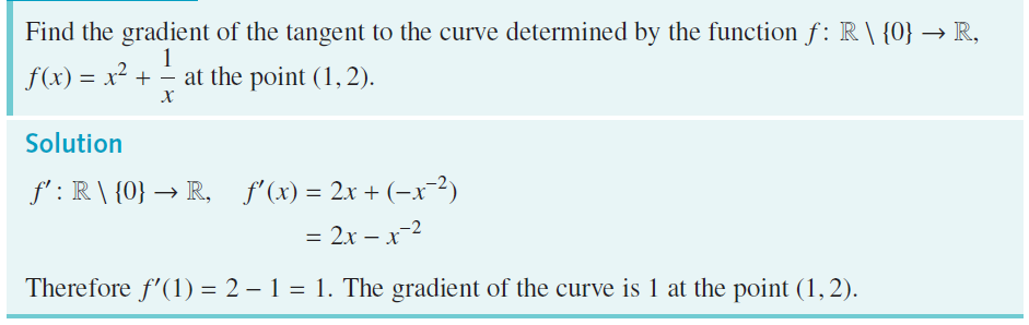
Worked example (own): Find the derivative of \(f(x) = 4x^{-3}\), stating the domain.
\(f'(x) = 4 \times (-3) \times x^{-4} = -12x^{-4}\), domain: \(x \neq 0\)
- Marks are commonly lost for giving the right derivative but forgetting to state "domain: x ≠ 0" — VCE markers want both.
- Don't confuse \(x^{-2}\) (which is \(1/x^2\)) with \(-x^2\) (which is negative \(x^2\)) — the sign and the power are different things.
Graphs of the Derivative Function
Plain English & method
This section asks you to go the other way: instead of computing f′(x) with algebra, you read the gradient straight off a picture of f(x) and sketch f′(x) from that.
The rule of thumb: walk along the curve of f(x) left to right and ask "is it going up, flat, or going down right now?"
- Where f(x) is increasing (sloping up), f′(x) is positive — plot it above the x-axis.
- Where f(x) is decreasing (sloping down), f′(x) is negative — plot it below the x-axis.
- Where f(x) has a stationary pointA point where the gradient is exactly zero — the tangent is horizontal. (a turning point, momentarily flat), f′(x) = 0 — plot it exactly on the x-axis.
The steeper the curve at a point, the further f′(x) sits from zero at that x-value; the flatter the curve, the closer f′(x) sits to zero.
Angle of a tangent: since gradient = tan(θ), where θ is the angle the tangent makes with the positive x-axis, you can also work backwards from an angle to a gradient value using m = tan(θ), then solve f′(x) = m.
Worked examples
Screenshot from class showing the sign-of-gradient table (increasing/decreasing/stationary) used to build up the shape of the derivative graph.
Worked examples: sketching a derivative graph from a given polynomial graph, and finding points where the tangent makes a given angle with the x-axis or is parallel to a given line.
- f′(x) = 0 marks an x-intercept on the derivative graph, not the height of the original function at that point — a very common mix-up.
- "Parallel to a line y = mx + c" means the gradient equals m — set f′(x) = m and solve for x.
Limits and Continuity
Plain English & method
A limitThe value a function approaches as x gets closer and closer to some number, whether or not the function is actually defined there. asks: as x sneaks up on some value a, what value does f(x) sneak up on? Notation: \(\lim_{x \to a} f(x)\).
Method 1 — direct substitution. If the function is defined at x = a, just plug a in. Most limits are this easy.
Method 2 — factorise first. If substituting gives the undefined form 0/0, that is a signal — not an error — that x = a is a common root of the top and bottom, so a matching factor can be cancelled before you substitute again.
Other substitution outcomes:
- Substituting gives (nonzero number)/0 → the limit does not exist (the function shoots off to infinity there).
- Substituting gives 0/(nonzero number) → the limit is 0.
Continuity and one-sided limits. A function is continuousYou can draw it without lifting your pen — no jumps, holes, or breaks. at x = a only if the limit from the left and the limit from the right both exist and are equal to each other (and to f(a)). If the left-hand limit and right-hand limit disagree, the function has a discontinuity at that point and \(\lim_{x \to a} f(x)\) does not exist overall — even though each one-sided limit might exist separately.
Building it from scratch (the Calculus Made Easy way)
"The value a function approaches" can sound vague until you actually watch it happen with real numbers. Take \(g(x) = (x^2 - 4)/(x - 2)\), and ask what happens as x sneaks up on 2 — without ever actually substituting x = 2 (which gives the undefined 0/0).
| x | 1.9 | 1.99 | 1.999 | → 2 ← | 2.001 | 2.01 | 2.1 |
|---|---|---|---|---|---|---|---|
| g(x) | 3.9 | 3.99 | 3.999 | ? | 4.001 | 4.01 | 4.1 |
Whichever side x creeps in from, g(x) is obviously homing in on exactly 4 — even though x = 2 itself is never plugged in and g(2) is technically undefined (0/0). That settling-down value, 4, is the limit. The algebra just gives you a shortcut to that same number without building a table every time:
This is exactly why 0/0 is treated as a "keep going" signal rather than a dead end: the function is perfectly well-behaved and predictable right up next to x = 2, it just happens to have a removable gap exactly at that one point — and factorising is simply the fastest way to see what value it's homing in on either side of that gap.
Worked examples
Class screenshots covering the substitution method and the 0/0-factorise method, plus the graph example showing left/right limits disagreeing at a discontinuity.
Worked examples: two limits solved by factorising a 0/0 form, and reading left-hand vs right-hand limits off a graph with a break at x = 1.
- 0/0 is not "the answer is 0" and not "undefined, stop here" — it specifically means "factorise and try again".
- When asked for a limit "as x → 1" on a graph with a jump at x = 1, check whether the question wants the left limit, the right limit, or the overall two-sided limit (which fails to exist if they differ).
When is the Function Differentiable?
Plain English & method
A function is differentiableIts derivative exists at that point — the curve has one single well-defined gradient there. at a point if the derivative actually exists there, formally: the limit that defines f′(x) exists at that x-value. For that to happen, the graph of f(x) has to be smooth at that point — no breaks, no sharp corners/cusps, and no vertical tangent.
Practically, look for three trouble spots:
- A break or hole in the graph (a discontinuity, straight from 17F) — not differentiable there, because the function isn't even continuous.
- A sharp corner/cusp (like the point of |x| at x = 0) — the gradient coming in from the left doesn't match the gradient leaving to the right, so there's no single gradient value to call the derivative.
- A vertical tangent — the gradient would be infinite, which isn't a real number, so the derivative doesn't exist there either.
When sketching f′(x), mark any of these x-values with an open dot on the derivative graph — the derivative graph has a genuine gap there, even if f(x) itself is unbroken (as at a sharp corner).
Worked examples
Class screenshots showing the identifying-features table for differentiability, plus example graphs of piecewise functions with a corner point.
Worked examples: sketching f′(x) with an open dot at a non-differentiable point, and finding the domain of f′(x) for a piecewise-defined function.
- A function can be perfectly continuous (no jumps) and still not be differentiable — a sharp corner is the classic case (think of the graph of |x|).
- "Not differentiable at x = a" does not mean f(a) is undefined — the function value can exist fine; it's the gradient that has no single value there.
Tangents and Normals
Plain English & method
The derivative gives you the gradient of the curve at a point. Once you have a gradient and a point, finding the equation of a line is just \(y - y_1 = m(x - x_1)\).
The tangent is the straight line that just touches the curve at that point and has the same gradient as the curve there: \(m_{tangent} = f'(x_1)\).
The normal is the line through the same point that is perpendicularMeeting at a right angle (90°). to the tangent. Two perpendicular gradients always multiply to −1, so:
Method, every time:
- Differentiate f(x) to get f′(x).
- Substitute the given x-value into f′(x) to get the gradient at that point.
- For the normal, flip and negate that gradient (m → −1/m).
- Substitute the point and the gradient into \(y - y_1 = m(x - x_1)\) and simplify.
Key ideas (from class)
Class key-ideas screenshot plus two worked examples on this exact method.

Worked examples
Worked examples straight from Haileybury notes: the tangent equation at (1, −1), the normal equation at the same point, and finding where tangents to a curve are parallel to a given line.
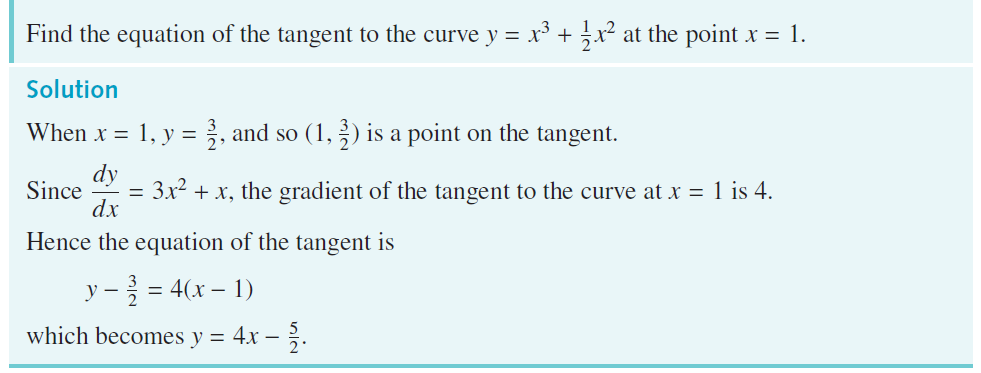
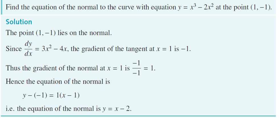
- The normal's gradient is the negative reciprocal of the tangent's — students very commonly just negate the gradient (forgetting to also flip it) or just flip it (forgetting to negate).
- "Parallel to the line y = mx + c" is a hint to set f′(x) = m and solve for x — the same trick as in 17D.
Rates of Change
Plain English & method
Two different, easily-confused ideas share the words "rate of change" in VCE Methods — know exactly which one a question is asking for.
Average rate of change (AROC) over an interval [a, b] is just the gradient of the straight line joining the two endpoints of the curve — how much the function changed overall, divided by how far x moved:
Instantaneous rate of change (IROC) at a single point x = a is the derivative evaluated there — the gradient of the tangent at that exact instant:
Sign tells you direction: f′(a) > 0 means the quantity is increasing at that instant; f′(a) < 0 means it's decreasing.
Key ideas (from class)
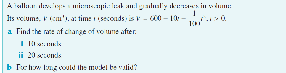
Class notes with the AROC formula and a worked balloon-volume problem (leaking balloon, volume decreasing over time).

Worked examples
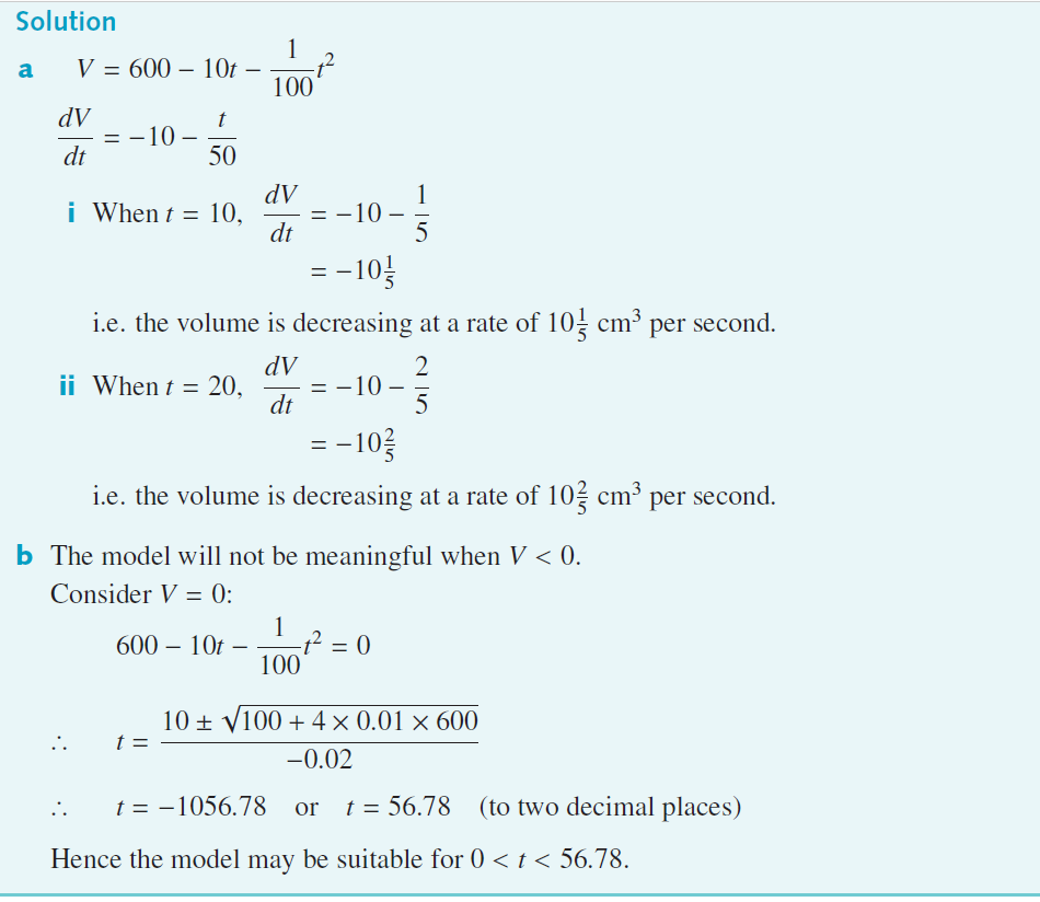
Worked examples: computing AROC over two different intervals and the IROC at a specific time for the same function, plus a real-world rate problem (a leaking balloon's volume) including checking when the model stops making physical sense.
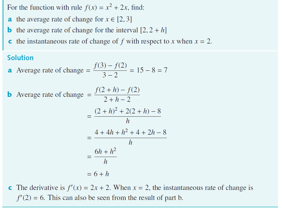
- AROC needs two points (an interval); IROC needs only one point and one derivative evaluation — mixing these up is the single most common error in this topic.
- "For how long could the model be valid?" style questions want you to notice when a quantity like volume would become negative — a model can be mathematically fine but physically meaningless outside some domain.
Stationary Points
Plain English & method
A stationary pointA point where the tangent to the curve is exactly horizontal — the gradient is momentarily zero. is any point on the curve where the gradient is zero — the tangent there is parallel to the x-axis (perfectly flat).
Method:
- Differentiate f(x) to get f′(x).
- Set f′(x) = 0 and solve for x — this may need factorising, the quadratic formula, or CAS.
- Substitute each x-value back into the original f(x) (not f′(x)!) to get the matching y-coordinate.
A cubic or quartic can have several stationary points — solving f′(x) = 0 finds all of them at once, since it's just solving an equation.
Building it from scratch (the Calculus Made Easy way)
Why does f′(x) = 0 find these points at all? Thompson's chapter on maxima and minima in Calculus Made Easy builds the idea from something you've physically felt, not from algebra first.
Step 1 — picture walking over a hill. Walking up the hill, your height is increasing with every step: the slope under your feet is positive. Walking down the far side, your height is decreasing: the slope is negative. Somewhere between "still going up" and "now going down" there has to be one exact spot — the summit — where, for a single instant, you are neither climbing nor descending. The ground under your feet is momentarily flat.
Step 2 — translate "flat" into calculus. "Flat" means the gradient is zero at that instant. Since f′(x) is the gradient of the curve at x, the summit (or, for a valley, the very bottom) is exactly where f′(x) = 0. That's the entire justification for the method in 18C: you're not being asked to memorise "set the derivative to zero", you're locating the flat spot(s) on the curve, the same way you'd feel a false-flat moment at the very top of a real hill.
Step 3 — this only finds candidates, not final answers. Setting f′(x) = 0 finds every place the curve goes flat — but a flat spot could be a peak, a valley, or (as in 18D) a "shelf" that isn't a peak or valley at all. That's exactly why 18D exists: finding the flat spots is only half the job, you still have to work out what kind of flat spot each one is.
Key ideas (from class)
Class notes and a labelled graph showing three stationary points (A, B, C) on one curve.

Worked examples
Worked examples: finding stationary point coordinates for two different polynomials, and a reverse problem — given that a curve has a stationary point at a known x-value, find an unknown coefficient in the function's rule.
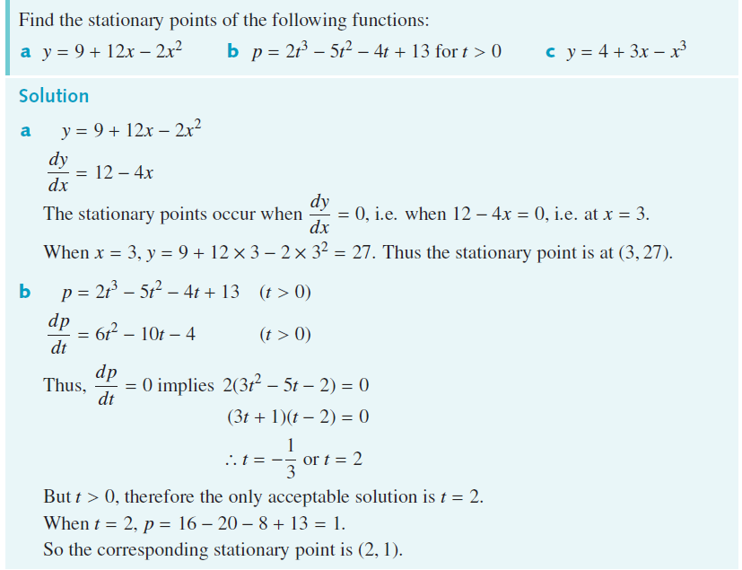
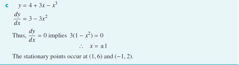
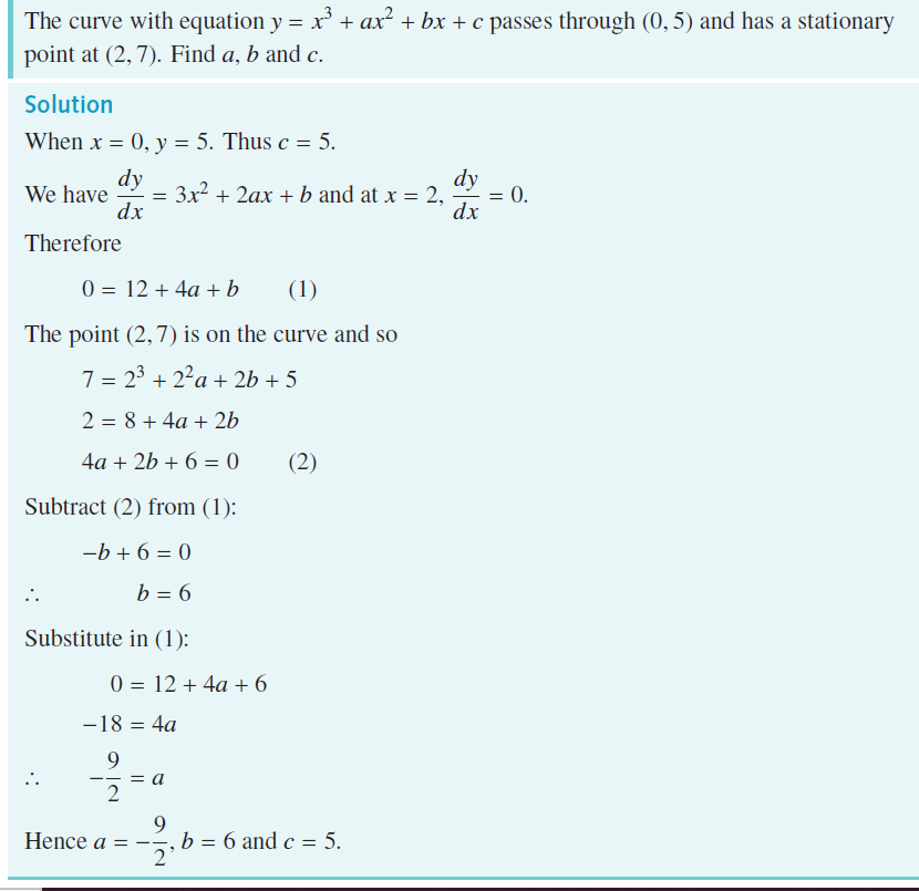
- The single most common slip in this whole chapter: after solving f′(x) = 0 for x, substituting back into f′(x) again instead of f(x) — this gives 0 for every point, which is meaningless as a y-coordinate.
- A stationary point is a coordinate pair (x, y) — always give both, not just the x-value.
Types of Stationary Points
Plain English & method
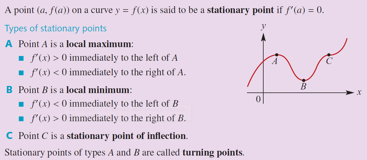
Finding a stationary point (18C) only tells you where the gradient is zero — it doesn't say what kind of point it is. There are three types:
- Local maximumA stationary point that is higher than the points immediately around it — a "peak". — gradient goes from positive to negative as x increases through the point (curve rises, flattens, falls).
- Local minimumA stationary point that is lower than the points immediately around it — a "trough". — gradient goes from negative to positive (curve falls, flattens, rises).
- Stationary point of inflectionA flat "shelf" in the curve where it keeps going in the same overall direction on both sides. — gradient has the same sign on both sides (positive→positive or negative→negative) — the curve flattens for an instant but keeps heading the same way.
Method — the sign diagram:
- Find the stationary point(s) as in 18C by solving f′(x) = 0.
- Pick a test x-value just to the left of the stationary point and one just to the right (not equal to the stationary x-value itself).
- Substitute each test value into f′(x) and record only its sign (+ or −), not the number.
- Read the pattern left→right against the three bullet points above to name the point.
Building it from scratch (the Calculus Made Easy way)
The sign-diagram method above is the one your class notes use, and it always works. Thompson's book teaches a second way of answering the same question — worth knowing as a mental cross-check, even if you write the sign diagram up for full marks.
Step 1 — recall what f′(x) > 0 and f′(x) < 0 mean. f′(x) is itself a function of x, with its own gradient — how quickly the gradient itself is changing. That "gradient of the gradient" is called the second derivativeWritten f″(x): the derivative of the derivative — how fast the gradient itself is changing., written f″(x).
Step 2 — connect that to the shape of a hill or valley. At the summit of a hill, the gradient goes from positive (climbing) to zero (the peak) to negative (descending) — the gradient itself is decreasing all the way through. A quantity whose own rate of change is decreasing has a negative second derivative. So:
Step 3 — the mirror image for a valley. At the bottom of a valley, the gradient goes from negative (descending) to zero to positive (climbing again) — the gradient itself is increasing. A positive second derivative:
Step 4 — the one case it can't decide. If f″(x) = 0 too at that point, the second derivative test is inconclusive — the point could still be a maximum, minimum, or inflection, and you have to fall back on the sign-diagram method from above to be sure. This is exactly why your class notes teach the sign diagram as the main method: it never has a "can't tell" case, while the second-derivative test occasionally does.
Worked example (own), to see both methods agree: for \(f(x) = x^3 - 3x\), \(f'(x) = 3x^2 - 3 = 0\) gives \(x=1\) and \(x=-1\). \(f''(x) = 6x\). At \(x=1\): \(f''(1) = 6 > 0\), so it's a local minimum. At \(x=-1\): \(f''(-1) = -6 < 0\), so it's a local maximum — matching whatever a sign diagram at those same two points would tell you.
Worked example (own) — the simplest possible point of inflection, and why the second-derivative test can go blank: for \(f(x) = x^3\), \(f'(x) = 3x^2 = 0\) gives \(x=0\) as the only stationary point. Trying the second-derivative test: \(f''(x) = 6x\), so \(f''(0) = 0\) too — this is exactly Step 4's \"can't decide\" case. Falling back to the sign diagram instead: pick \(x=-1\) (\(f'(-1) = 3 > 0\)) and \(x=1\) (\(f'(1) = 3 > 0\)) — positive on both sides, so \(x=0\) is a stationary point of inflection, not a max or min. Picture it as a flat landing halfway up a single continuous flight of stairs: the curve pauses to go perfectly flat for an instant at x = 0, but it was climbing before and keeps climbing after — it was never a peak or a valley, just a brief flattening on the way up.
Key ideas (from class)
Class notes and worked examples building sign diagrams, plus a full sketch (intercepts + stationary points) example.
Worked examples
Worked examples: classifying every stationary point of a given function using a sign diagram, sketching a full graph with y-intercepts, x-intercepts and stationary points all marked, and finding the interval(s) where a function is increasing.
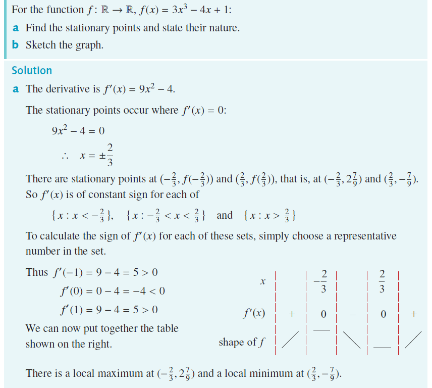
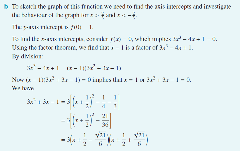
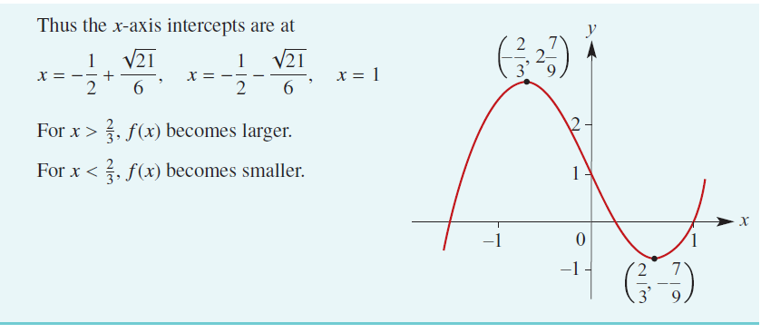
- "Increasing on this interval" means f′(x) > 0 throughout that interval — this connects straight back to 17D's sign-of-gradient idea.
- Don't skip the test-value step and guess the shape from the leading term alone — the sign diagram is what actually earns the marks, and it catches inflection points that are easy to miss by eye.
Applications to Maximum and Minimum Problems
Plain English & method
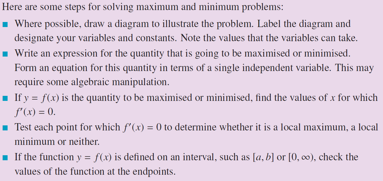
This is where calculus starts solving real problems: "what dimensions give the biggest volume", "what's the cheapest way to build this". The calculus (18C + 18D) is the easy part — the hard part is turning the words into a function of one variable.
Standard method:
- Draw a diagram and label the changing quantities with variables.
- Write down the quantity you want to optimise (volume, area, cost…) as a function — it will usually start with two variables, connected by a constraint the question gives you (e.g. a fixed amount of material/area).
- Use the constraint to eliminate one variable, leaving a single-variable function, e.g. V(x).
- Work out the valid domain for x from the physical setup — lengths can't be negative, and there's often an upper limit too.
- Differentiate, set the derivative to 0, solve, and check it's a maximum or minimum with a sign diagram (18D).
- Answer the actual question asked — often "what is the maximum value" (substitute back into the original function), not just the x-value that produces it.
Endpoint maxima/minima — the twist to watch for. Calculus only finds local turning points. If the domain is restricted (e.g. 0 ≤ x ≤ 0.3), the true absolute maximumThe single highest value the function actually reaches anywhere across its whole domain — not just at a local turning point. or absolute minimumThe single lowest value the function actually reaches anywhere across its whole domain. might occur at the edge of the domain instead of at a stationary point. Always check the function's value at both endpoints of the domain and compare them against any stationary points found inside it.
Key ideas (from class)
Class notes with a canvas-shelter volume problem and a folded-box volume problem, including the endpoint-restriction twist on the box problem.
Worked examples
Two full worked applications from your notes: a canvas shelter with 24 m² of material (maximise enclosed volume), and a 2 m square sheet of metal folded into an open box (maximise volume, then re-solve with a height restriction of 0.3 m forcing an endpoint check).
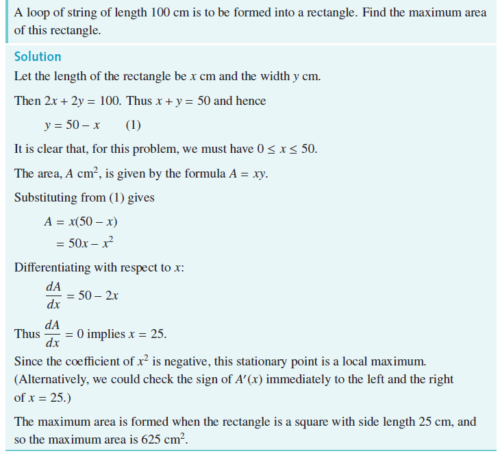
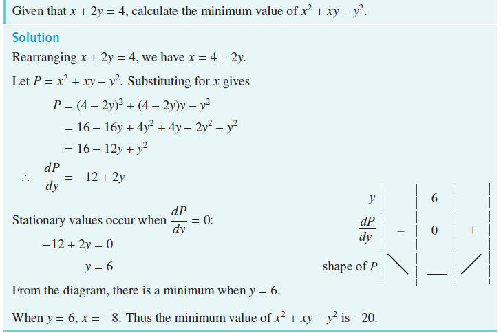
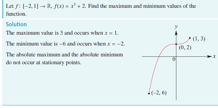
- Forgetting step 4 (working out the valid domain) is the most common way marks are lost here — a maximum that comes out at a negative length or an impossible dimension is a sign the domain wasn't restricted properly.
- When a domain restriction is added partway through a question, always re-check whether the true maximum/minimum has moved to an endpoint rather than assuming the original stationary point still wins.
Applications of Differentiation to Kinematics
Plain English & method
KinematicsThe study of motion — here, always a single particle moving along a straight line. in this course means one particle moving along a straight line, and differentiation is the tool that connects position, velocity, and acceleration.
\(v(t) = x'(t)\) = velocity (the first derivative of position)
\(a(t) = v'(t) = x''(t)\) = acceleration (the second derivative of position)
Two quantities that sound similar but aren't the same:
- DisplacementPosition relative to a fixed origin O — it's a vector, so it has a sign/direction. is a vector (has direction) — it can be negative, meaning "on the other side of the origin".
- Distance is a scalar (no direction) — it's always positive, and it's the total length actually travelled, which is not the same as the net displacement if the particle changes direction along the way.
Reading the sign of velocity and acceleration:
- v(t) > 0 → moving in the positive direction; v(t) < 0 → moving in the negative direction; v(t) = 0 → instantaneously at rest.
- a(t) > 0 → speeding up in the positive sense; a(t) < 0 → slowing down (or speeding up in the negative sense); a(t) = 0 → travelling at constant velocity.
Key ideas (from class)
Class notes covering the displacement/velocity/acceleration definitions, the displacement-time and velocity-time graph gradients, and worked examples.

Worked examples
Multi-part worked examples from your notes on particles moving in a straight line: finding when velocity/acceleration is zero and what the other quantity equals at that instant, finding total distance travelled, and working out for how long the velocity stays negative.
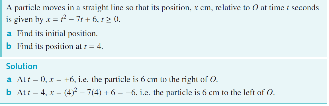
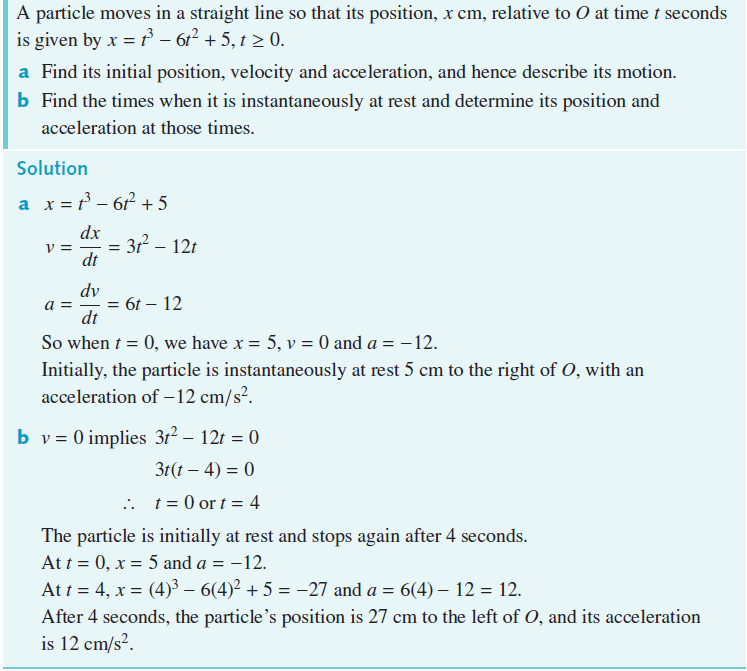
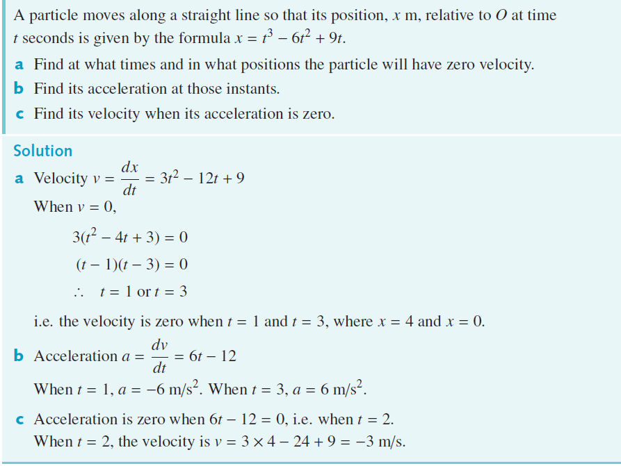
- "Distance travelled" is not the same as "displacement" the moment the particle changes direction at some point — you have to split the motion into the parts before and after it turns around and add up the distances for each part separately.
- Velocity is the FIRST derivative and acceleration is the SECOND derivative of position — mixing up the order is an easy but costly slip under exam pressure.
Families of Functions and Transformations
Plain English & method
Note: the Canvas page for this lesson on your school's system is broken — it's an accidental duplicate of the 18F kinematics page (same images, same content), so there was no usable class material to pull from here. The explanation below is written from scratch to cover the standard VCE Methods topic this lesson title refers to, so this gap doesn't leave you unprepared if it does come up.
A "family of functions" just means a group of related graphs built from one base function by transforming it — shifting it, stretching it, or flipping it. The question this lesson answers: if you know how f(x) was transformed into a new function, what happens to its derivative?
The key fact: transformations applied vertically (up/down shifts, vertical stretches) and transformations applied horizontally (left/right shifts, horizontal stretches) affect the derivative differently.
- Vertical translation — g(x) = f(x) + c: adding a constant shifts the whole graph up or down but doesn't change its steepness anywhere, so g′(x) = f′(x) exactly, unchanged. (This is the same fact as "the derivative of a constant is 0" from 17B, just viewed graphically.)
- Vertical dilation — g(x) = k·f(x): stretching the graph vertically by factor k also stretches every gradient by the same factor: g′(x) = k·f′(x).
- Horizontal translation — g(x) = f(x − h): shifting the graph sideways by h shifts its derivative graph sideways by the same amount: g′(x) = f′(x − h).
- Horizontal dilation — g(x) = f(ax): scaling x by a factor also scales the derivative by that same factor (this one follows from the chain rule in 20A: differentiating f(ax) with u = ax gives g′(x) = a·f′(ax)).
- Reflection in the x-axis — g(x) = −f(x): flips the sign of the gradient everywhere: g′(x) = −f′(x).
Practically, exam questions in this style usually show you a graph of f(x) (or describe a transformation in words) and ask you to identify or sketch the matching transformation of f′(x) — which is really just 17D's "read the gradient off the graph" skill, applied to a shifted or scaled picture instead of the original.
Worked examples
No usable key-ideas image exists for this lesson (see note above).
No class worked examples exist for this lesson (see note above) — see the original worked example below instead.
Worked example (own): If \(f(x)\) has derivative \(f'(x) = 3x^2\), find \(g'(x)\) for \(g(x) = 2f(x-1) + 5\).
- The "+5" is a vertical translation — it disappears entirely when differentiating.
- The "2×" is a vertical dilation — it carries straight through as a factor of 2.
- The "(x − 1)" is a horizontal translation — it carries straight through unchanged (no extra scaling, since horizontal translations don't introduce a multiplier, only horizontal dilations do).
\(g'(x) = 2f'(x-1) = 2 \times 3(x-1)^2 = 6(x-1)^2\)
- Vertical changes to f(x) (shifting up/down, or the constant term) do NOT change f′(x)'s shape, only vertical changes that involve scaling do.
- Horizontal changes to f(x) DO change f′(x), and a horizontal dilation also introduces a scaling factor on top of the shift — it's not a pure 1-for-1 transformation like the vertical translation case.
The Chain Rule
Plain English & method
Some functions, like \(y = (3x^2 + 1)^{-1}\) or \(y = (x^3 + 1)^3\), are one function nested inside another — a "function of a function", called a composite functionA function built by feeding the output of one function into another, e.g. \(y = (x^3+1)^3\) is "cube it" applied to "\(x^3+1\)".. Expanding a bracket like \((x^3+1)^3\) by hand to differentiate term-by-term is slow and error-prone. The chain rule differentiates composite functions directly, without expanding anything.
The method: substitute an inner function as u.
- Spot the "inside" expression (what's inside the brackets, or under a root, or in a denominator) and call it u.
- Rewrite y purely in terms of u — this is now a simple power of u.
- Differentiate y with respect to u (dy/du), and separately differentiate u with respect to x (du/dx).
- Multiply the two derivatives together — that product is dy/dx.
Worked example, straight from the class video (20A): differentiate \(y = (x^3 + 1)^3\).
- Let \(u = x^3 + 1\), so \(y = u^3\).
- \(\dfrac{dy}{du} = 3u^2\) and \(\dfrac{du}{dx} = 3x^2\).
- Chain rule: \(\dfrac{dy}{dx} = \dfrac{dy}{du} \times \dfrac{du}{dx} = 3u^2 \times 3x^2 = 9x^2(x^3+1)^2\).
Second worked example, also from the class video: find the gradient of \(y = \dfrac{16}{3x^2+1}\) at the point \((1, 4)\).
- Rewrite as a negative power first: \(y = 16(3x^2+1)^{-1}\).
- Let \(u = 3x^2+1\), so \(y = 16u^{-1}\).
- \(\dfrac{dy}{du} = -16u^{-2}\) and \(\dfrac{du}{dx} = 6x\).
- \(\dfrac{dy}{dx} = -16u^{-2} \times 6x = -96x(3x^2+1)^{-2}\).
- Substitute \(x=1\) (so \(u = 3(1)^2+1 = 4\)): \(\dfrac{dy}{dx} = -96(1)(4)^{-2} = -\dfrac{96}{16} = -6\). The gradient at \((1,4)\) is \(-6\).
Building it from scratch (the Calculus Made Easy way)
Thompson calls the chain rule "a useful dodge" in Calculus Made Easy, and that word choice is the whole point: it isn't a new law of calculus, it's a clever trick for avoiding painful algebra you already know how to do — just slowly.
The motivating problem. Try to differentiate \(y = (x^2 + c)^3\) using only what you knew before the chain rule. You'd have to expand the cube of a bracket, collect terms, and differentiate a five-term polynomial — doable, but slow, and it gets worse for higher powers or messier brackets. The dodge sidesteps all of that expansion.
Step 1 — name the "inside" expression u. For \(y = (x^2+c)^3\), let \(u = x^2+c\). Now \(y\) is simply \(u\) cubed:
Step 2 — differentiate each simple piece on its own. Both of these are ordinary power-rule differentiations, nothing new:
Step 3 — multiply the two rates together. This is the one genuinely new idea, and it's worth understanding rather than memorising: dy/dx measures "how fast does y change as x changes", and that overall rate is built from two smaller rates chained together — how fast y changes as u changes, times how fast u changes as x changes.
Why multiply, not add? The classic picture (used by Thompson and by pretty much every calculus teacher since, because it works) is interlocking gears. If gear A turns the input and gear B is driven by gear A, and gear B turns twice as fast as gear A for every full turn A makes, while gear C (driven by B) turns three times as fast as B — then C turns 2 × 3 = 6 times as fast as A overall. Rates that are chained one inside another compound by multiplying, not adding, and that's exactly the structure of a composite function: x drives u, and u drives y.
Notice this derivation slots straight into the worked examples above — the same u-substitution, the same "differentiate each piece, then multiply" pattern, just with \(u = x^3+1\) or \(u = 3x^2+1\) instead of \(x^2+c\). Once you've built it once by hand, the shortcut stops feeling like an arbitrary rule to memorise.
Worked examples
No textbook key-ideas screenshot was posted for this lesson on Canvas (it's video-only) — the formula and both worked examples above were reconstructed from the class lecture video.
The two worked examples above are directly from the 20A lecture video, reconstructed frame-by-frame.
- The single most common chain rule error: multiplying dy/du by du/dx but leaving u un-substituted back to an x-expression in the final answer — always finish by replacing u with what it stands for.
- Rewrite roots and fractions as powers first (\(\sqrt{x} = x^{1/2}\), \(1/x^2 = x^{-2}\)) before trying to identify u — it's much easier to spot the "inside function" once everything is in index form.
Differentiating Rational Powers
Plain English & method
A rational powerA power written as a fraction, e.g. x^(1/2), which is the same thing as a root: x^(1/2) = √x. is just a fraction sitting in the exponent — and the good news is the exact same power rule from 17B/17C still applies with no changes: bring the power down, subtract 1 from it. The only extra care needed is fraction arithmetic when subtracting 1 from a fractional power.
Worked example, straight from the class video (20B): differentiate \(f(x) = 4x^{2/3}\).
- Bring down the power: \(4 \times \dfrac{2}{3} = \dfrac{8}{3}\).
- Subtract 1 from the power: \(\dfrac{2}{3} - 1 = \dfrac{2}{3} - \dfrac{3}{3} = -\dfrac{1}{3}\).
- \(f'(x) = \dfrac{8}{3}x^{-1/3}\), which can also be written as \(\dfrac{8}{3x^{1/3}}\) or \(\dfrac{8}{3\sqrt[3]{x}}\).
Second worked example, also from the class video: differentiate \(f(x) = x^{1/5}\).
- Bring down the power: \(1 \times \dfrac{1}{5} = \dfrac{1}{5}\).
- Subtract 1 from the power: \(\dfrac{1}{5} - 1 = \dfrac{1}{5} - \dfrac{5}{5} = -\dfrac{4}{5}\).
- \(f'(x) = \dfrac{1}{5}x^{-4/5}\).
When the inside isn't just x — e.g. differentiating something like \((x^2+1)^{1/2}\) (which is \(\sqrt{x^2+1}\)) — the power is fractional and there's a composite function, so 20A's chain rule and 20B's fractional power rule combine: treat it exactly like a chain-rule problem (\(u = x^2+1\)), just with a fractional power on u.
Worked examples
No textbook key-ideas screenshot was posted for this lesson on Canvas either (also video-only) — the rule and both worked examples above were reconstructed from the class lecture video.
Both worked examples above are directly from the 20B lecture video, reconstructed frame-by-frame.
- Fraction subtraction under exam pressure (2/3 − 1) is where most marks are actually lost in this topic, not the calculus itself — always rewrite 1 with the same denominator first (3/3, 5/5, etc.) before subtracting.
- \(\sqrt{x}\) is \(x^{1/2}\), not \(x^2\) — mixing up a root and a square is a very easy slip when converting notation before differentiating.
Cram sheet — every formula in one place
One-screen reference for the night before. If you can explain why each line works, not just recite it, you're in good shape.
| Topic | Formula / rule |
|---|---|
| 16C Average rate of change | \(\text{AROC on }[a,b] = \dfrac{f(b)-f(a)}{b-a}\) — the chord's gradient |
| 16D Instantaneous rate of change | Draw the tangent and measure its gradient, or use a very short chord as an estimate |
| 16E Average velocity | \(\dfrac{x(t_2)-x(t_1)}{t_2-t_1}\) — position-time graph gradient = velocity |
| 17B/17C Power rule | \(f(x)=ax^n \implies f'(x)=a n x^{n-1}\) (state domain \(x \neq 0\) if \(n\) is negative) |
| 18A Tangent | \(y - y_1 = f'(x_1)(x-x_1)\) |
| 18A Normal | \(m_{normal} = \dfrac{-1}{f'(x_1)}\) |
| 18B Average rate of change | \(\text{AROC on }[a,b] = \dfrac{f(b)-f(a)}{b-a}\) |
| 18B Instantaneous rate of change | \(\text{IROC at } x=a \text{ is } f'(a)\) |
| 18C Stationary points | Solve \(f'(x)=0\), then sub \(x\) back into \(f(x)\) for the y-coordinate |
| 18D Classify stationary point | Sign diagram of \(f'(x)\): \(+\to-\) local max, \(-\to+\) local min, same sign both sides = inflection |
| 18E Max/min problems | Constraint → single-variable function → domain → \(f'(x)=0\) → check endpoints too |
| 18F Kinematics | \(x(t)\) position, \(v(t)=x'(t)\) velocity, \(a(t)=v'(t)=x''(t)\) acceleration |
| 20A Chain rule | \(\dfrac{dy}{dx} = \dfrac{dy}{du}\times\dfrac{du}{dx}\) (let \(u\) = the "inside" expression) |
| 20B Rational powers | \(f(x)=ax^{p/q} \implies f'(x)=a\left(\dfrac{p}{q}\right)x^{(p/q)-1}\) — same power rule, watch the fraction arithmetic |
- Forgetting to write "domain: x ≠ 0" after a negative-power derivative.
- Substituting a stationary x-value back into f′(x) instead of f(x) for the y-coordinate.
- Getting the normal gradient by only flipping OR only negating, not both.
- Mixing up displacement (signed, can be negative) with distance travelled (always positive, total path length).
- Not checking domain endpoints in a restricted max/min problem.
Video resources — watch in this order
Curated and link-checked, grouped by chapter, in a sensible watch order (foundations before applications). These supplement the portal — they don't replace working through the lessons and worked examples above.
Foundations — what a derivative actually is (watch first)
Chapter 16 — Rates of Change (prerequisite foundation)
Chapter 17 — Differentiation of Polynomials
Chapter 18 — Applications of Differentiation
Chapter 20 — Chain Rule & Rational Powers
Exam-ready — the last step
Every video above teaches the mechanics. The single best last step before Monday is your own school's "MM Unit 2 Practice Test — Differentiation" (tech-free + tech-active sections, with the official solutions) — it's already sitting in your Test Revision folder on Canvas, and it's the exact format, timing, and difficulty of the real thing. Do it timed, mark it against the solutions, then come back to whichever lesson tab above covers whatever you got wrong.